1.4 — Ricardian One-Factor Model
ECON 324 • International Trade • Fall 2020
Ryan Safner
Assistant Professor of Economics
safner@hood.edu
ryansafner/tradeF20
tradeF20.classes.ryansafner.com
A Note of Caution and A Judgment Call
Feenstra and Taylor dive right into a Ricardian model in Ch. 2 with some advanced features; Ch. 4 is H-O Model
- A lot of moving parts are thrown at you rather quickly
In my experience (and from using other textbooks), it's better to build up slowly:
- Simplified Ricardian model
- Standard "neoclassical model" (not in F&T)
- H-O Model
So if you are reading the textbook, it won't exactly match up to class for 1-2 weeks 😕

Assumptions of the Ricardian One-Factor Model
Assumptions of the One-Factor Model
- Markets (both output and factors) are perfectly competitive
- “Labor” is homogenous and non-specific
- Labor is mobile domestically, but not internationally
- Production of goods requires only varying amounts of labor as an input
- The “one factor”
- The marginal product of labor is constant
- No barriers to trade or transactions costs
- Technology is constant within each country
- Resource endowments are fixed

Setting up the Model
Imagine 2 countries, Home and Foreign
Each country can produce two goods, xylophones (x) and yams (y)
Each country has a fixed total supply of labor
- L for Home and L′ for Foreign
Let:
- lx: amount of labor to make 1 x
- ly: amount of labor to make 1 y

Setting up the Model: Home
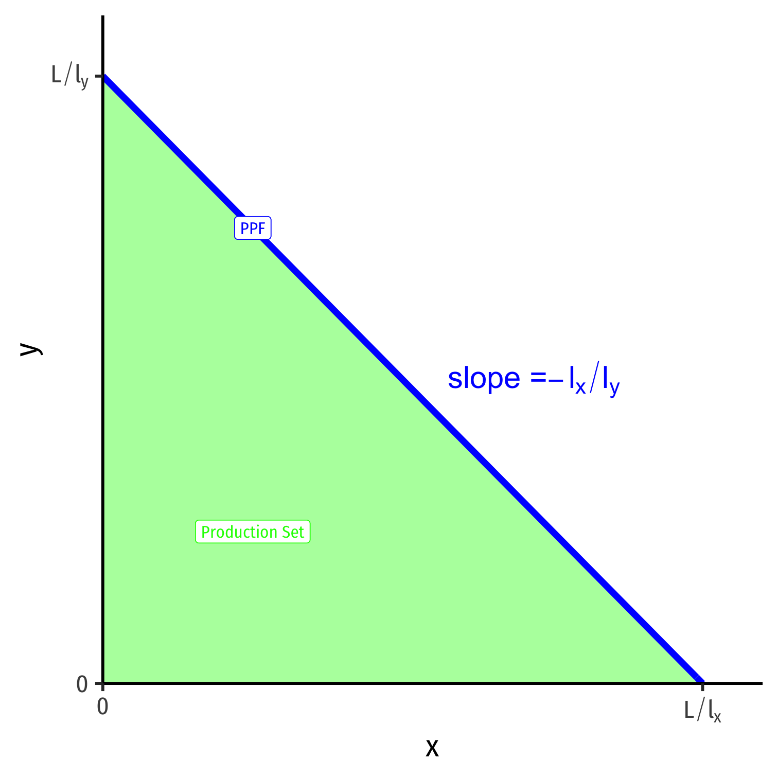
- Home's production set and total possible allocations of labor within a country is:
lxx+lyy≤L
- To find the frontier (PPF), assume Labor Demand (left) and Labor Supply (right) are equal:
lxx+lyy=L
Setting up the Model: Home
lxx+lyy=L
- Solve for y to graph
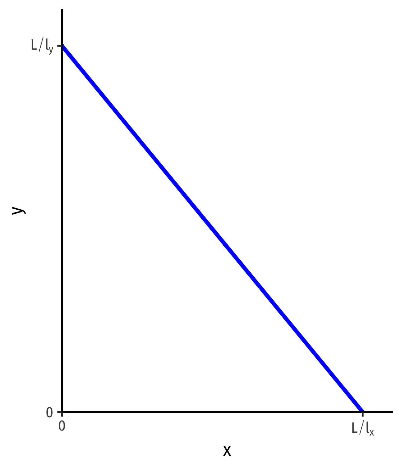
y=Lly−lxlyx
Setting up the Model: Home
lxx+lyy=L
- Solve for y to graph
y=Lly−lxlyx
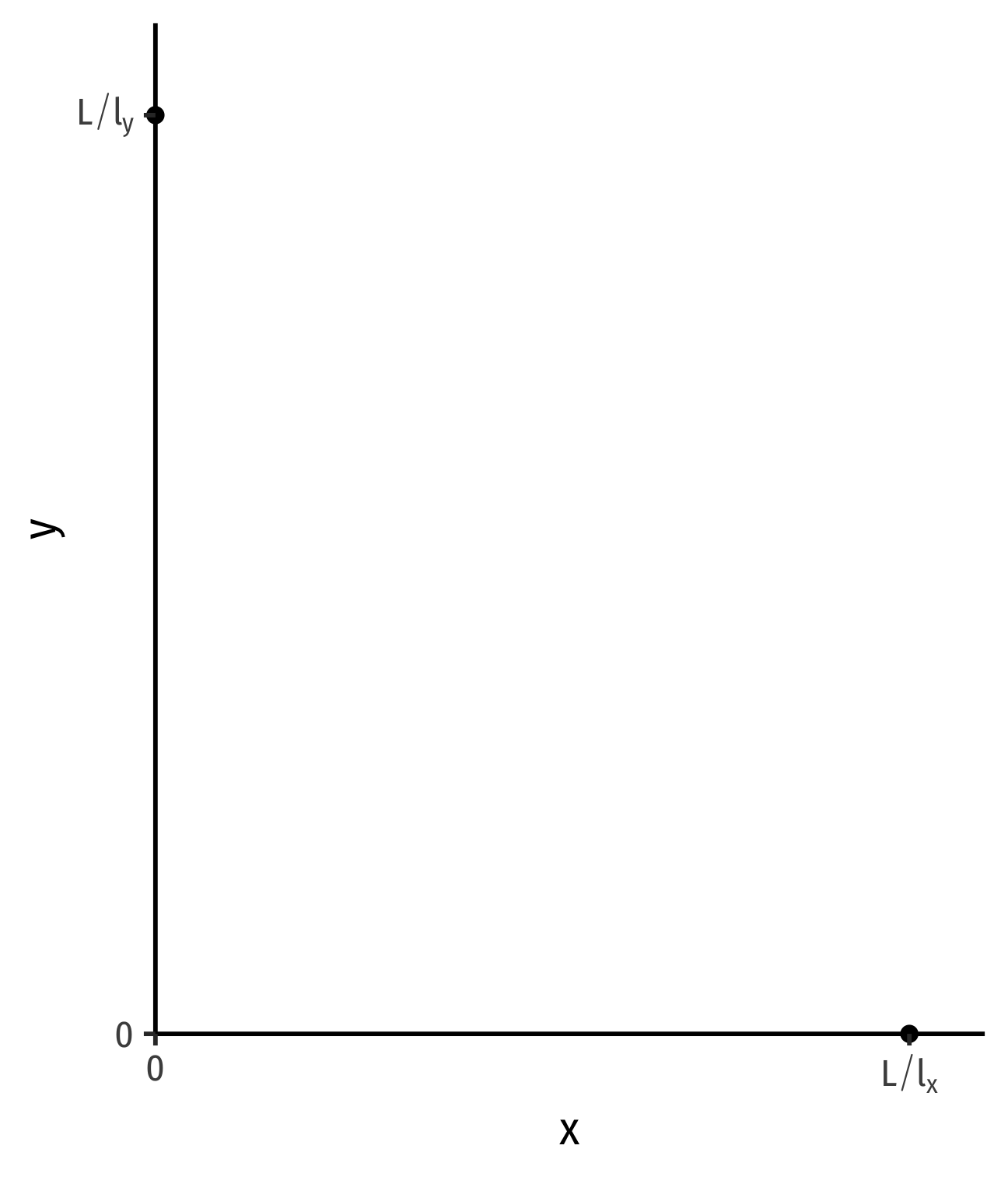
- y-intercept: Lly (max y production)
- x-intercept: Llx (max x production)
Setting up the Model: Home
lxx+lyy=L
- Solve for y to graph
y=Lly−lxlyx
- y-intercept: Lly (max y production)
- x-intercept: Llx (max x production)
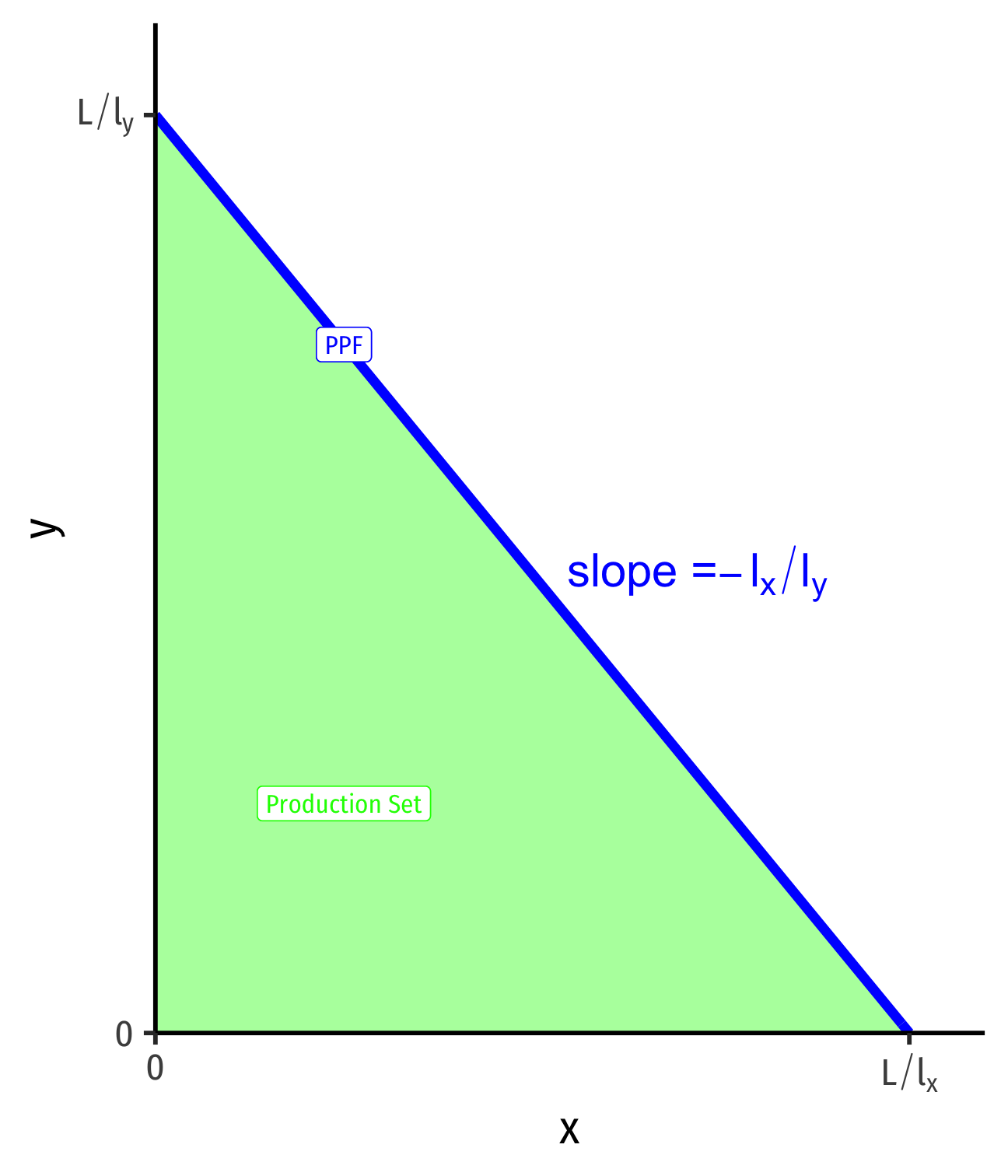
- slope: −lxly
Setting up the Model: Home
lxx+lyy=L
- Solve for y to graph
y=Lly−lxlyx
- y-intercept: Lly (max y production)
- x-intercept: Llx (max x production)
- slope: −lxly
Same As Before
Points on the frontier are efficient (uses all available labor supply)
Points beneath the frontier are feasible (in production set) but inefficient (does not use all available labor supply)
Points above the frontier are impossible with current constraints (labor supply, technology, trading opportunities)

Understanding the Tradeoff
Slope of PPF: marginal rate of transformation (MRT)
Rate at which (domestic) market values tradeoff between goods x and y
Relative price of x (in terms of y), or opportunity cost of x: how many units of y must be given up to produce one more unit of x
Absolute and Comparative Advantages (Autarky)
Absolute Advantage
A country has an absolute advantage if it requires less labor to produce (a unit of) a good
Examples:
- if lx<l′x, then Home has an absolute advantage in producing x
- if ly>l′y, then Foreign has an absolute advantage in producing y

Comparative Advantage
A country has a comparative advantage in a producing a good if the opportunity cost of producing that good is lower than other countries
Recall the slope of PPF (the MRT) is the relative price (opp. cost) of x
Examples:
- if lxly<l′xl′y, then Home has a comparative advantage in producing x
- if lxly>l′xl′y, then Foreign has a comparative advantage in producing x

Comparative Advantage, Some Hints
PPF slope = opportunity cost of good x (amount of y given up per 1 x)
If countries have different PPF slopes, have different opportunity costs
Comparative Advantage, Some Hints
PPF slope = opportunity cost of good x (amount of y given up per 1 x)
If countries have different PPF slopes, have different opportunity costs
Country with flatter slope (smaller magnitude) has lower opportunity cost of x (or higher cost of y) implies a comparative advantage in x
Country with steeper slope (larger magnitude) has higher opportunity cost of x (or lower cost of y) implies a comparative advantage in y
An Example in Autarky
Ricardian One-Factor Model Example
Example: Suppose the following facts to set up:
Home has 100 Laborers
- Requires 1 worker to make x
- Requires 2 workers to make y
Foreign has 100 Laborers
- Requires 1 worker to make x
- Requires 4 workers to make y
Ricardian One-Factor Model Example
Example: Suppose the following facts to set up:
Home has 100 Laborers
- Requires 1 worker to make x
- Requires 2 workers to make y
Foreign has 100 Laborers
- Requires 1 worker to make x
- Requires 4 workers to make y
For each country, find the equation of the PPF and graph it.
Which country has an absolute advantage in producing x and y?
Which country has an comparative advantage in producing x and y?
Ricardian One-Factor Model Example: Solving for PPFs
Home
lxx+lyy=L
Foreign
Ricardian One-Factor Model Example: Solving for PPFs
Home
lxx+lyy=L1x+2y=100
Foreign
Ricardian One-Factor Model Example: Solving for PPFs
Home
lxx+lyy=L1x+2y=1002y=100−x
Foreign
Ricardian One-Factor Model Example: Solving for PPFs
Home
lxx+lyy=L1x+2y=1002y=100−xy=50−0.5x
Foreign
Ricardian One-Factor Model Example: Solving for PPFs
Home
lxx+lyy=L1x+2y=1002y=100−xy=50−0.5x
Foreign
l′xx+l′yy=L′
Ricardian One-Factor Model Example: Solving for PPFs
Home
lxx+lyy=L1x+2y=1002y=100−xy=50−0.5x
Foreign
l′xx+l′yy=L′1x+4y=100
Ricardian One-Factor Model Example: Solving for PPFs
Home
lxx+lyy=L1x+2y=1002y=100−xy=50−0.5x
Foreign
l′xx+l′yy=L′1x+4y=1004y=100−x
Ricardian One-Factor Model Example: Solving for PPFs
Home
lxx+lyy=L1x+2y=1002y=100−xy=50−0.5x
Foreign
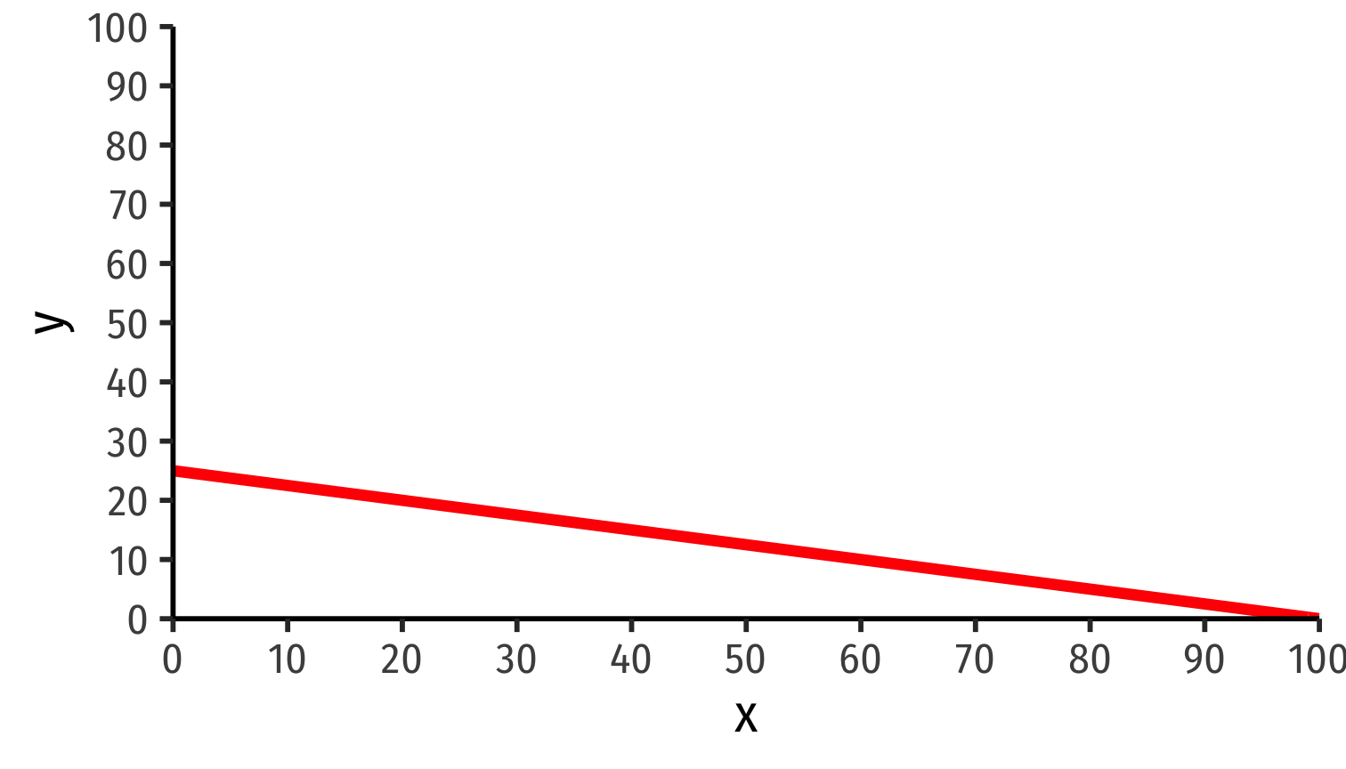
l′xx+l′yy=L′1x+4y=1004y=100−xy=25−0.25x
Ricardian One-Factor Model Example: Graphing PPFs
Home

y=50−0.5x
Foreign

y=25−0.25x
Example: Absolute Advantage
Home

lx=1
ly=2
Foreign
l′x=1
l′y=4
Example: Absolute Advantage
Home

lx=1 (Equal)
ly=2 (Absolute advantage)
Foreign

l′x=1 (Equal)
l′y=4 (Absolute disadvantage)
Comparative Advantage and Autarky Relative Prices
So far, we assume countries are in autarky, they are not trading with one another
To find comparative advantage for each country, we need to compare opportunity costs of producing each good in each country, or relative prices in autarky
A country with a lower autarky relative price of a good than another country has a comparative advantage in producing that good

Example: Comparative Advantage
Home
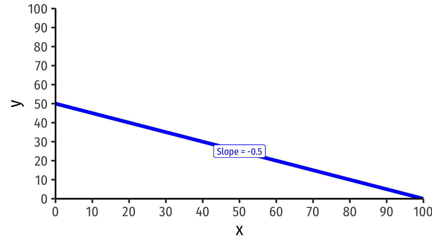
Autarky relative price of x: 0.5y [PPF slope!]
Autarky relative price of y: 2x
Foreign
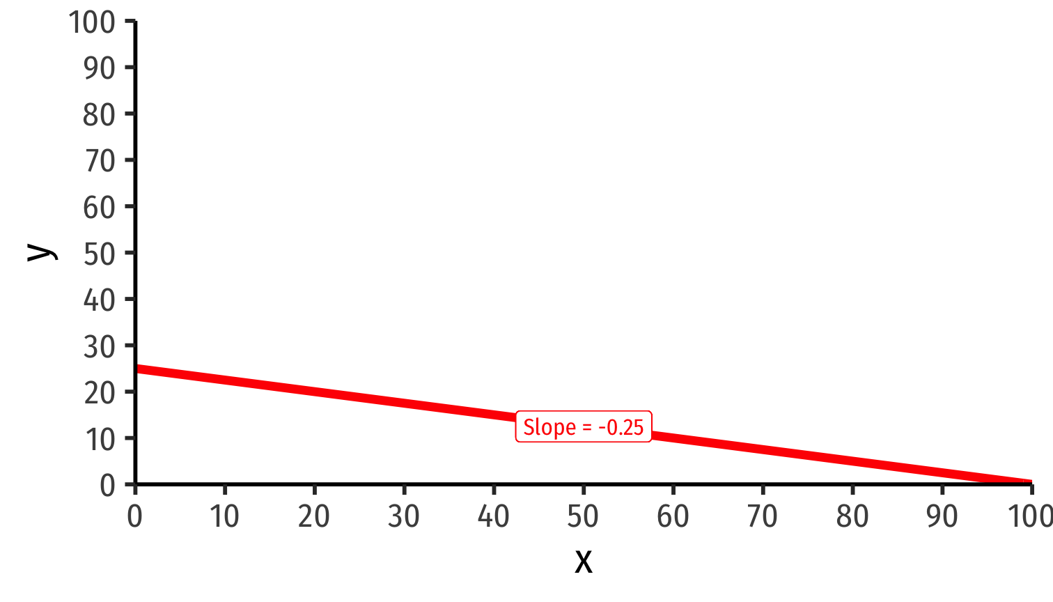
Autarky relative price of x: 0.25y [PPF slope!]
Autarky relative price of y: 4x
Example: Comparative Advantage
Autarky Relative Prices (Opportunity Costs)
| 1x | 1y | |
|---|---|---|
| Home | 0.5y | 2x |
| Foreign | 0.25y | 4x |
Example: Comparative Advantage
Autarky Relative Prices (Opportunity Costs)
| 1x | 1y | |
|---|---|---|
| Home | 0.5y | 2x |
| Foreign | 0.25y | 4x |
Home has a comparative advantage in producing y
Foreign has a comparative advantage in producing x
Example: Opening up Trade
Autarky Relative Prices (Opportunity Costs)
| 1x | 1y | |
|---|---|---|
| Home | 0.5y | 2x |
| Foreign | 0.25y | 4x |
Suppose now countries open up trade
We considered the relative prices in autarky
We next need to consider what might relative prices be under international trade
The Example with International Trade
Example: Opening up Trade
Autarky Relative Prices (Opportunity Costs)
| 1x | 1y | |
|---|---|---|
| Home | 0.5y | 2x |
| Foreign | 0.25y | 4x |
A bit of handwaiving here:
Ricardo assumes a labor theory of value and constant marginal products of labor
We have hidden the MPL† for simplicity here
We are also in direct exchange (barter) between goods, there is no money here
Suffice it to say that we can show that the ratio of labor requirements (PPF slope) is equal to the ratio of prices of the final goods: lxly⏟slope=pxpy
- a clearer explanation of this with our next model!
Example: Opening up Trade
Autarky Relative Prices (Opportunity Costs)
| 1x | 1y | |
|---|---|---|
| Home | 0.5y | 2x |
| Foreign | 0.25y | 4x |
Home will:
- buy x if px<0.5y
- sell y if py>2x
The autarky price of y:
- At Home: 2x
- In Foreign: 4x
Home can export y to Foreign and sell at higher price!
- All L in Home will move to (higher-paying) y industry
Example: Opening up Trade
Autarky Relative Prices (Opportunity Costs)
| 1x | 1y | |
|---|---|---|
| Home | 0.5y | 2x |
| Foreign | 0.25y | 4x |
Foreign will:
- sell x if px>0.25y
- buy y if py<4x
The autarky price of x:
- At Home: 0.5y
- In Foreign: 0.25y
Foreign can export x to Home and sell at higher price!
- All L' in Foreign will move to (higher-paying) x industry
Example: Opening up Trade
Autarky Relative Prices (Opportunity Costs)
| 1x | 1y | |
|---|---|---|
| Home | 0.5y | 2x |
| Foreign | 0.25y | 4x |
Possible range of world relative prices:
0.25y<px<0.5y
2x<py<4x
Example: Specialization
Home
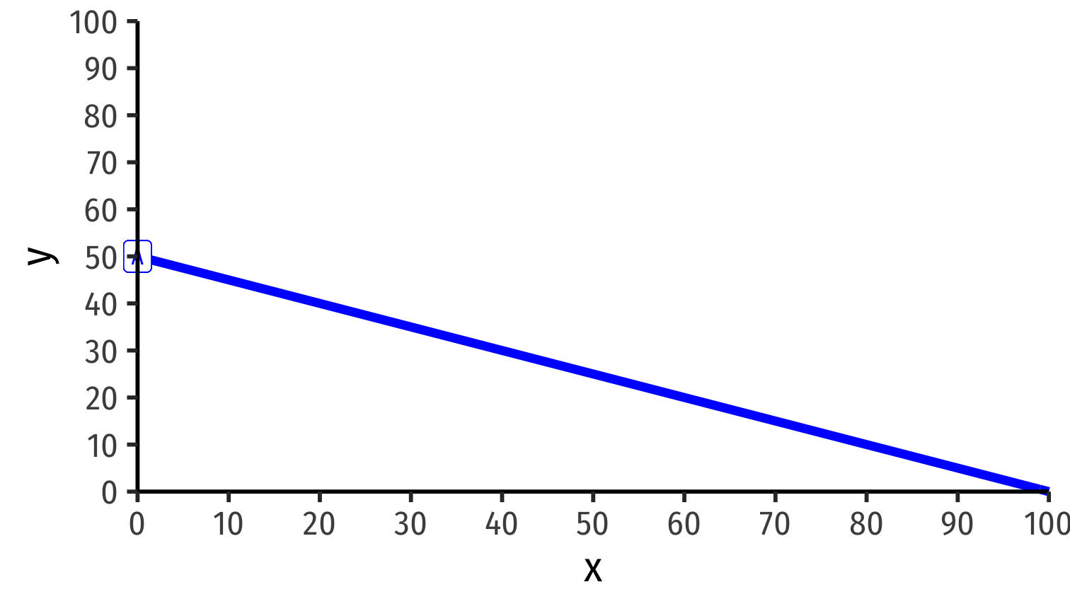
Home specializes in only producing y at point A
Foreign
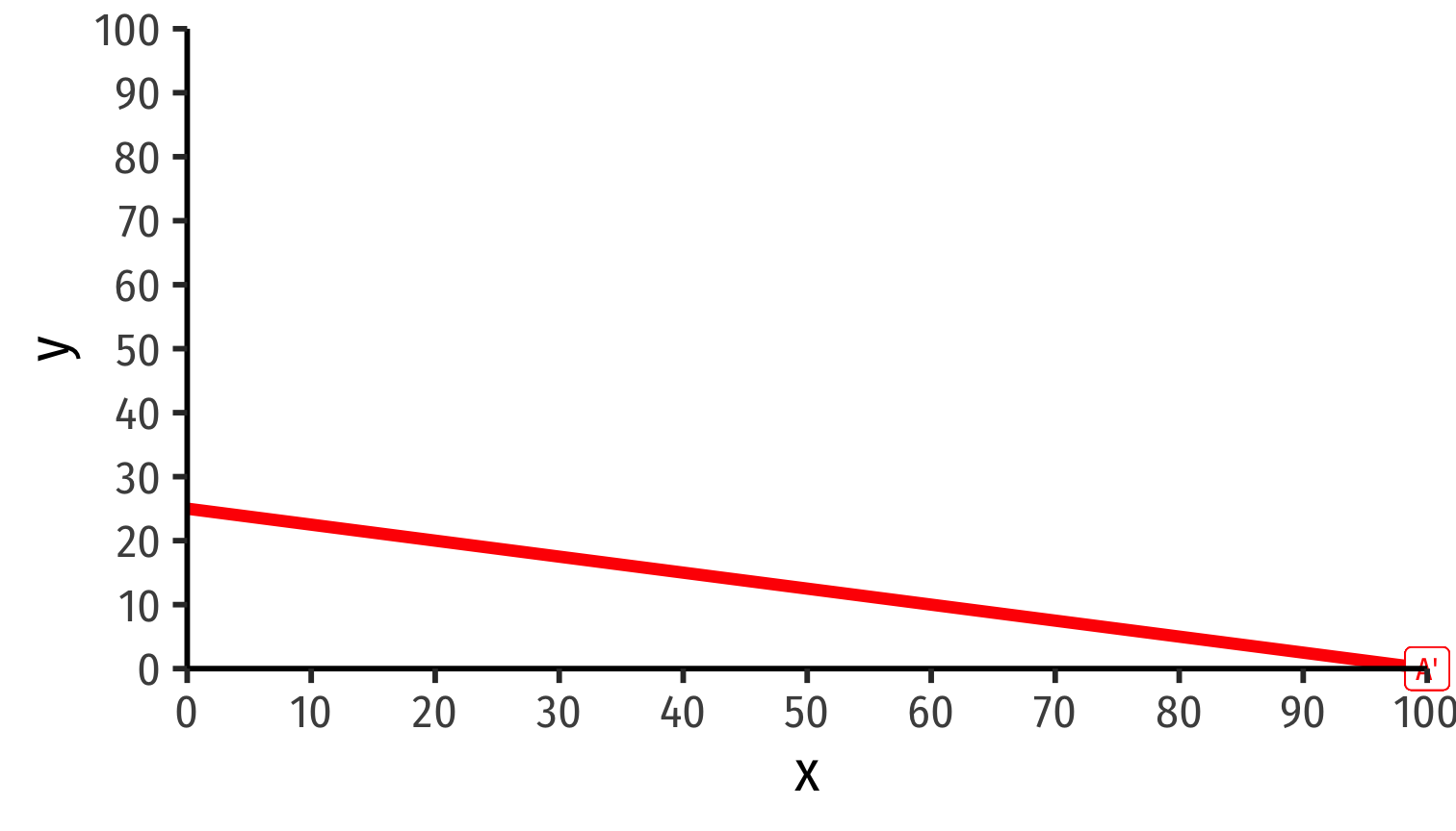
Foreign specializes in only producing x at point A'
International Trade Equilibrium: Price Adjustments
- Home exports y ⟹ less y sold in Home ⟹ ↑py in Home
International Trade Equilibrium: Price Adjustments
Home exports y ⟹ less y sold in Home ⟹ ↑py in Home
As y arrives in Foreign ⟹ more y sold in Foreign ⟹ ↓py in Foreign
International Trade Equilibrium: Price Adjustments
Home exports y ⟹ less y sold in Home ⟹ ↑py in Home
As y arrives in Foreign ⟹ more y sold in Foreign ⟹ ↓py in Foreign
Foreign exports x ⟹ less x sold in Foreign ⟹ ↑px in Foreign
International Trade Equilibrium: Price Adjustments
Home exports y ⟹ less y sold in Home ⟹ ↑py in Home
As y arrives in Foreign ⟹ more y sold in Foreign ⟹ ↓py in Foreign
Foreign exports x ⟹ less x sold in Foreign ⟹ ↑px in Foreign
As x arrives in Home ⟹ more x sold in Home ⟹ ↓px in Home
International Trade Equilibrium: World Relative Prices
- International trade equilibrium: relative prices adjust so they equalize across countries
p⋆xp⋆y=pxpy=p′xp′y
Must be within mutally agreeable range: 0.25y<px<0.5y
2x<py<4xSuppose the world relative price of x settles to p⋆xp⋆y=0.4y

International Trade Equilibrium: World Relative Prices
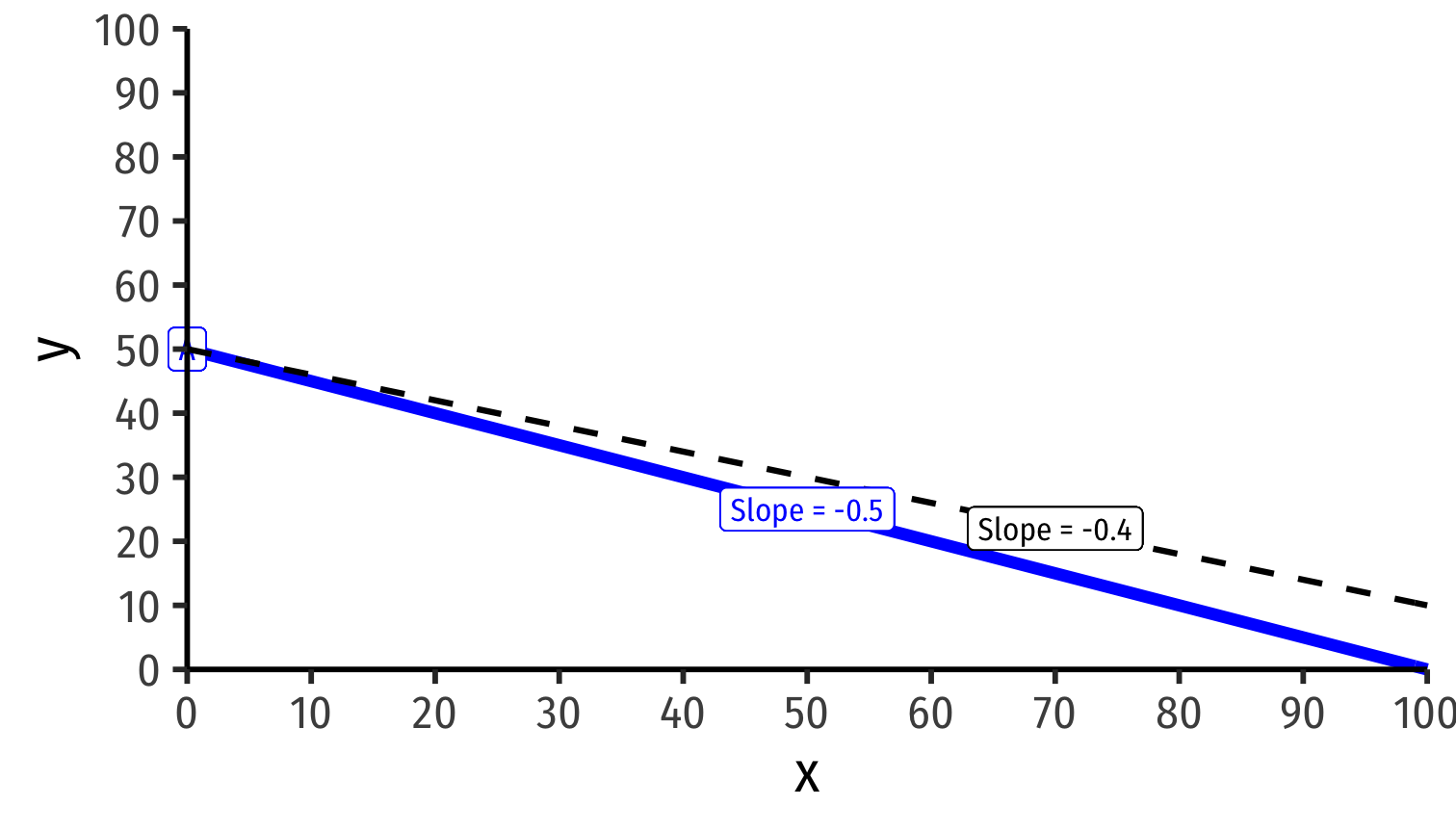
Home
Foreign
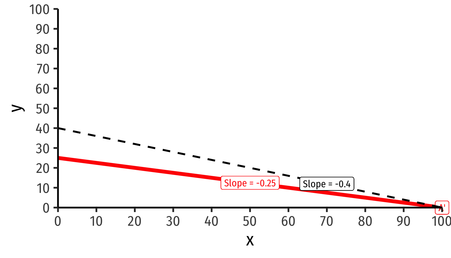
World relative price of x: p⋆xp⋆y=0.4y
Both countries face same international exchange rate with slope =−0.4
International Trade Equilibrium: “Trade Triangles”
Home
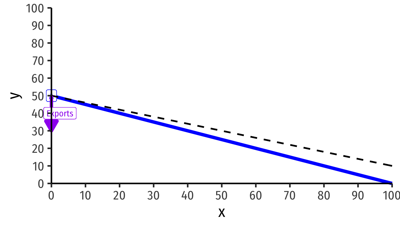
Home exports 20y to Foreign
Foreign
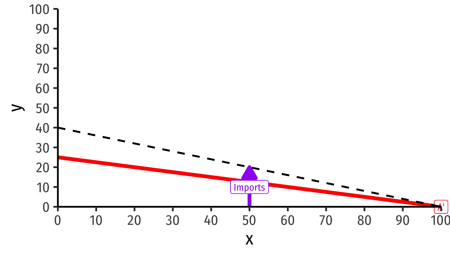
International Trade Equilibrium: “Trade Triangles”
Home

Home exports 20y to Foreign
Foreign exports 50x to Home
Foreign
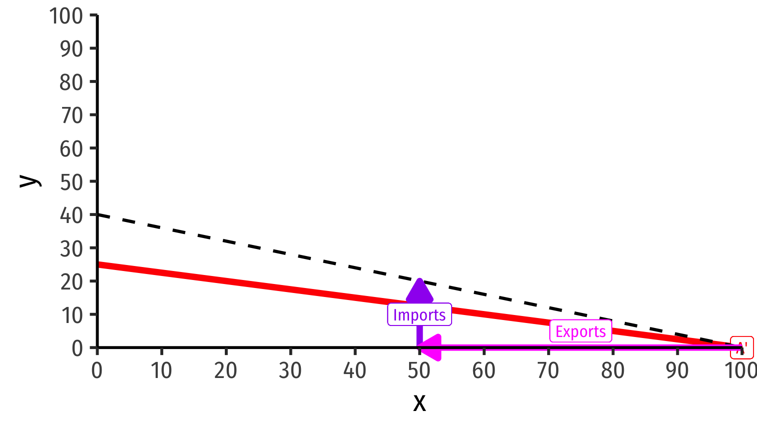
International Trade Equilibrium: “Trade Triangles”
Home
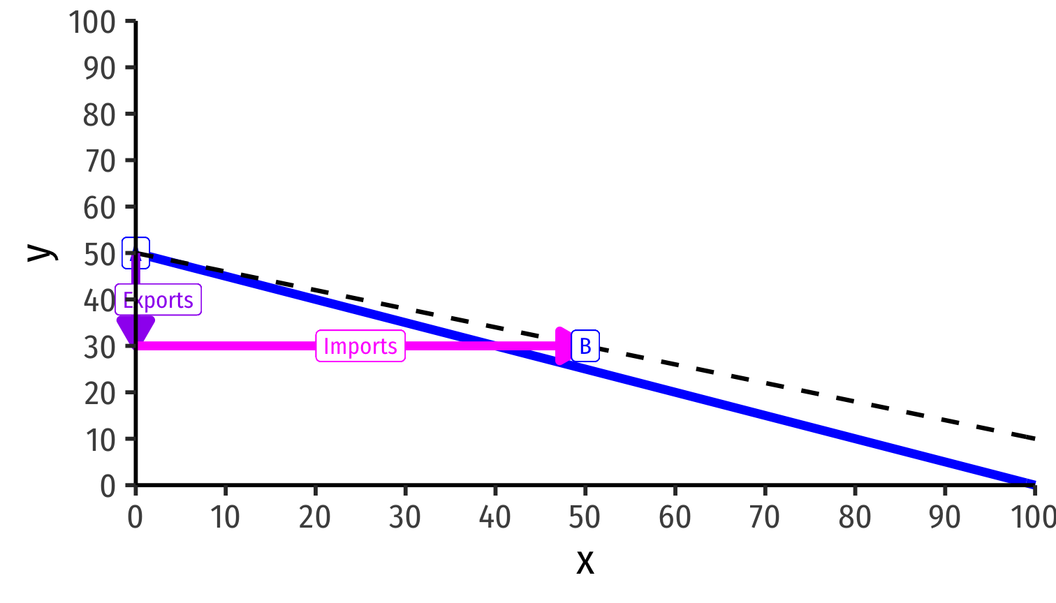
Foreign
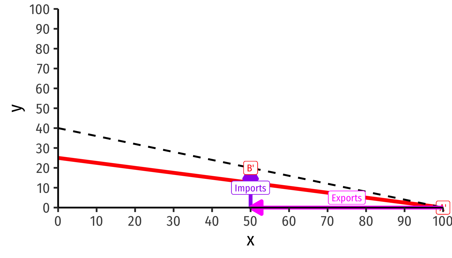
Trade along world exchange rate (world relative prices) from specialization points (A and A') to consumption points (B and B') beyond PPFs!
Another Example: You Try!
Example: Suppose the following facts to set up:
Home has 100 Laborers
- Requires 5 workers to make wheat
- Requires 10 workers to make cars
Foreign has 200 Laborers
- Requires 2 workers to make wheat
- Requires 8 workers to make cars
Plot wheat (w) on the horizontal axis and cars (c) on the vertical axis.
For each country, find the equation of the PPF and graph it.
Which country has an absolute advantage in producing wheat and cars?
Which country has an comparative advantage in producing wheat and cars?
What will the range of possible terms of trade be?