1.8 — The Specific Factors Model
ECON 324 • International Trade • Fall 2020
Ryan Safner
Assistant Professor of Economics
safner@hood.edu
ryansafner/tradeF20
tradeF20.classes.ryansafner.com
Assumptions of the Specific Factors Model
Assumptions of the Specific Factors Model
Until now, we've assumed (within each country), factors are mobile
But in truth, some factors are specific or immobile: can only be used for the production of a specific set of goods or industry
- e.g. programmers can only work in software, not in pro-football
- e.g. equipment used to make beer barrels cannot switch to producing computer chips
Opening up trade will affect the distribution of income between fixed and mobile factors

Assumptions of the Specific Factors Model
Imagine 2 countries, Home and Foreign
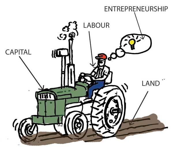
Countries have three factors of production:
- labor (L)
- capital (K)
- land (T)
Assumptions of the Specific Factors Model
Each country has two industries, manufacturing (M) and agriculture (A)
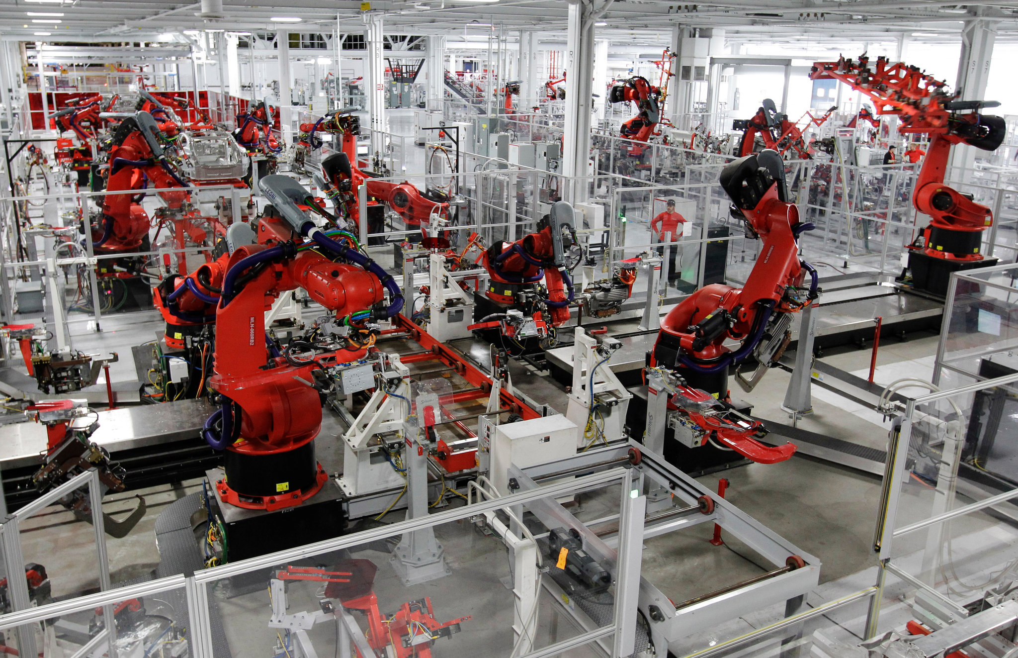
Manufacturing is produced using capital and labor
Agriculture is produced using land and labor
Land and capital are specific factors, only used to produce one good
Labor is the mobile factor that can be used in either (or both) sectors

Setting up the Model: Production Function
- An economy's production can be described as a set of production functions for manufacturing (m) and agriculture (a)
QM=QM(K,LM)QA=QA(T,LA)
- Each country can only allocate its labor force between two industries
LM+LA=ˉL


Diminishing Marginal Product of Labor
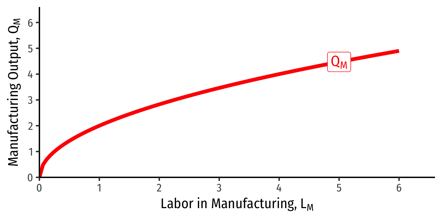
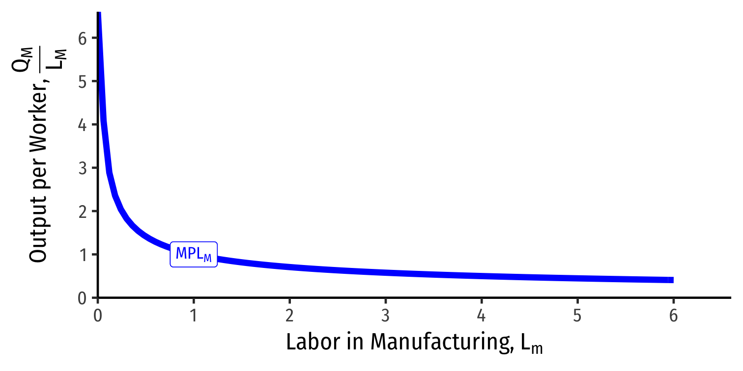
Each industry exhibits diminishing returns to labor
Marginal product of labor in manufacturing (MPLM): additional manufacturing output produced by adding one more unit of labor (holding K constant)
MPLM=ΔQMΔLM
- Declines as more L is added to manufacturing production
Diminishing Marginal Product of Labor
Each industry exhibits diminishing returns to labor
Marginal product of labor in agriculture (MPLA): additional agriculture output produced by adding one more unit of labor (holding T constant)
MPLA=ΔQAΔLA
- Declines as more L is added to agriculture production
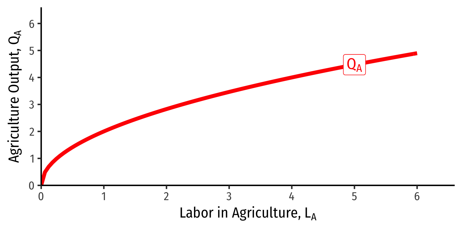
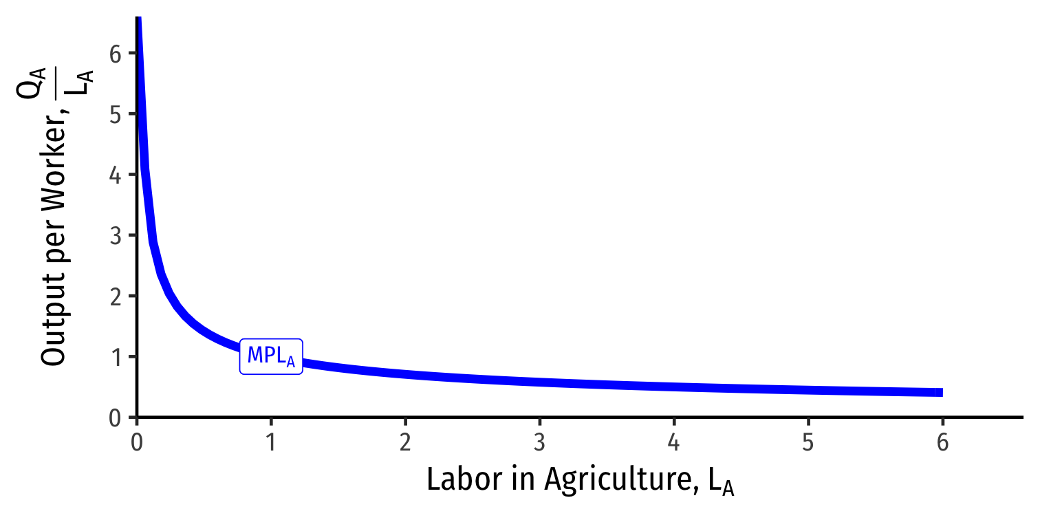
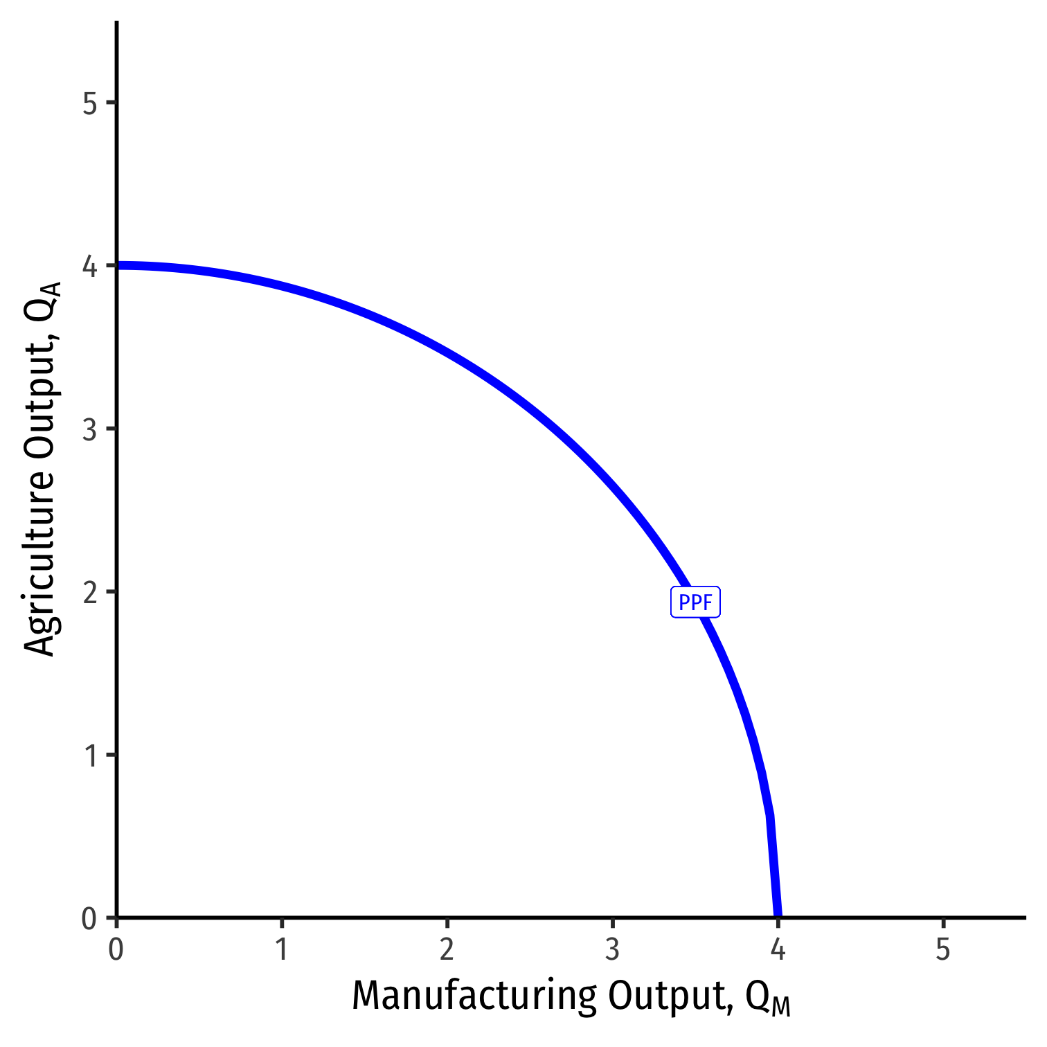
PPF
We get a PPF with increasing costs again
Let's examine more why
Allocating the Mobile Factor (Labor)
A Note About Labor
- A simple (and very Ricardian) assumption about labor: it is measured in hours, and can equally be applied to each industry
ˉL=LM+LA
Every labor hour allocated to agriculture is a labor hour not allocated to manufacturing, and vice versa
- Opportunity cost of labor
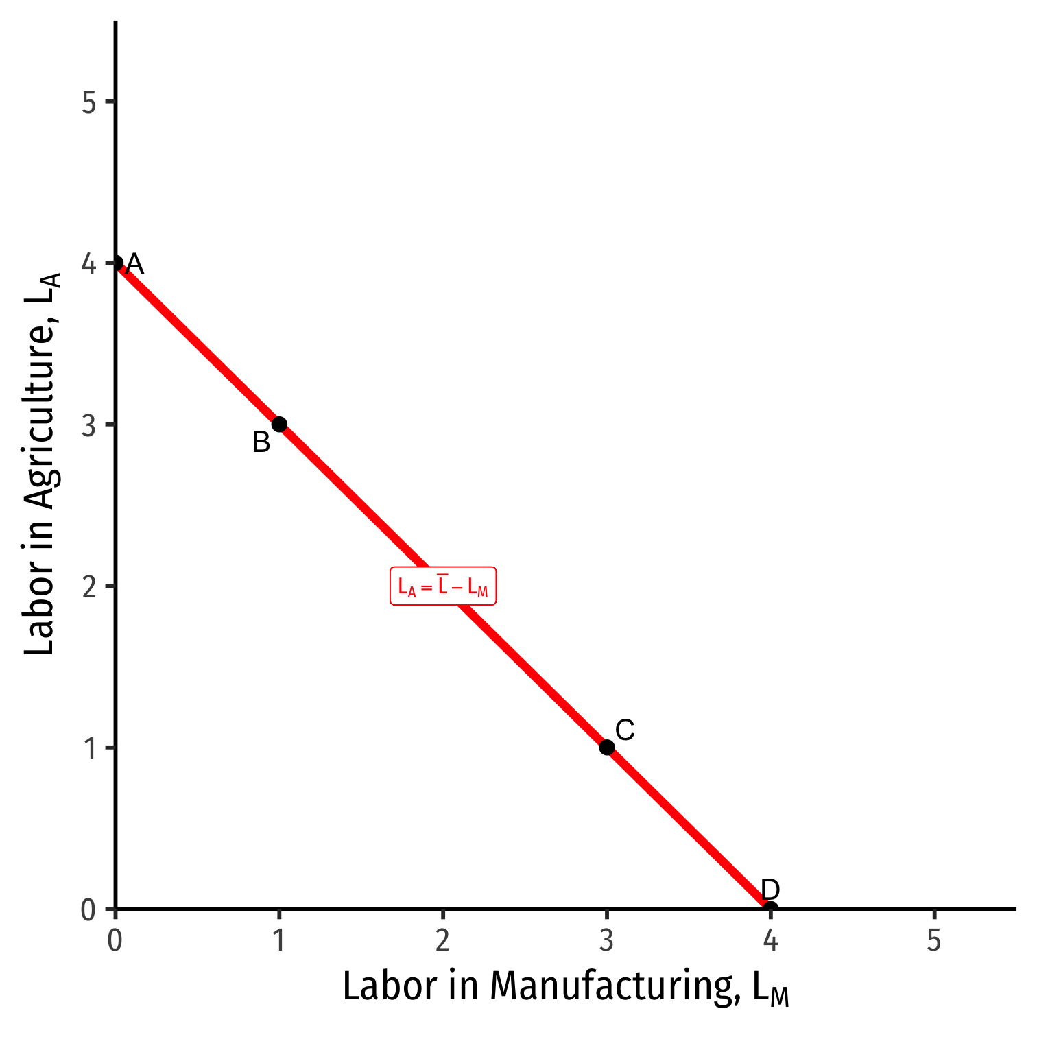
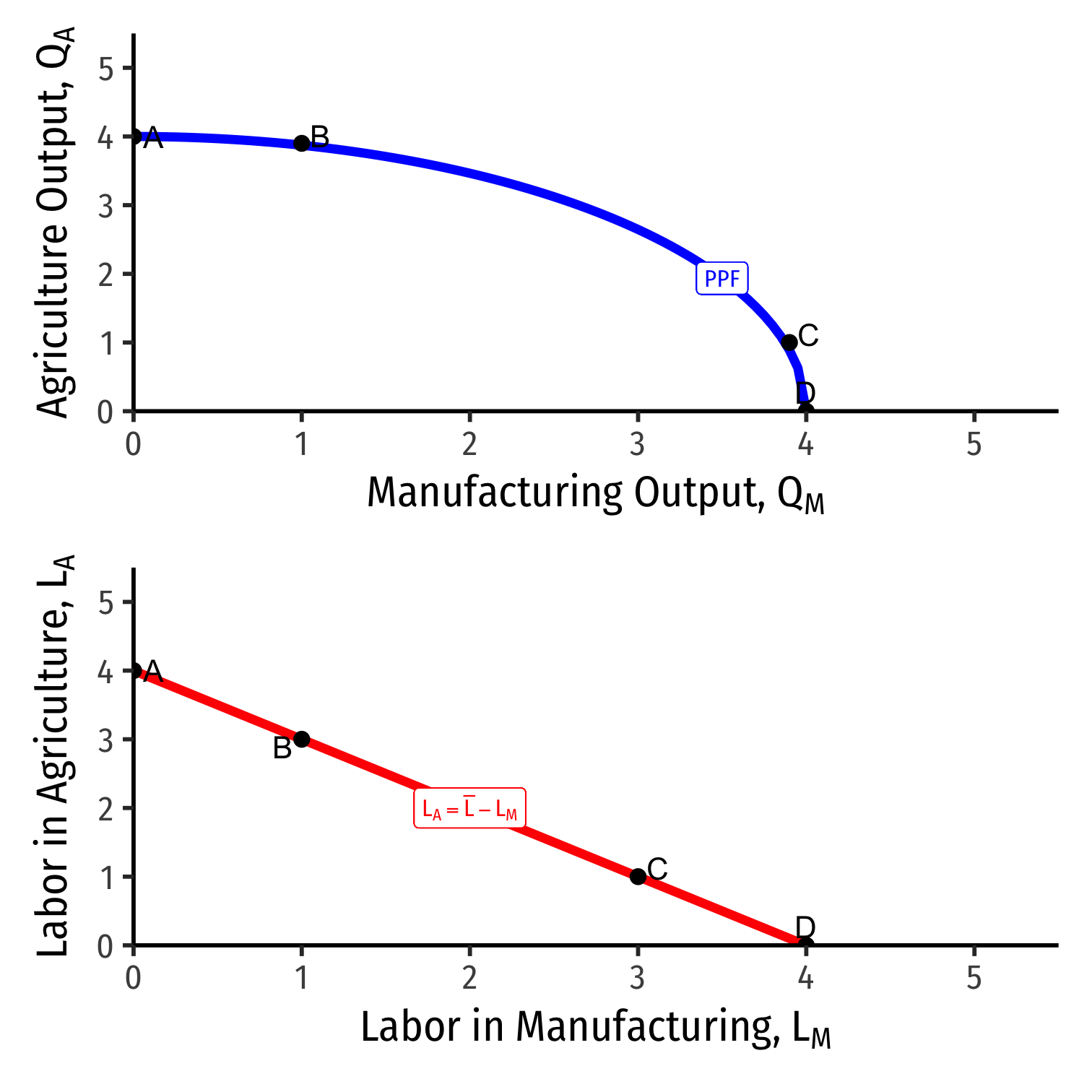
Visualize a “labor budget constraint” to understand movements along the PPF
Allocating Labor
Shows relationship of moving along PPF ⟺ reallocating labor across industries
If all labor in A (point A), country only produces A, no M
If all labor in M (point D), country only produces M, no A
Remember, each industry has diminishing returns to labor, and will have a particular MPL depending on how much land or capital there are
- Hence, a 1 unit ↑↓ in L in one industry does not imply a 1 unit increase

Allocating Labor
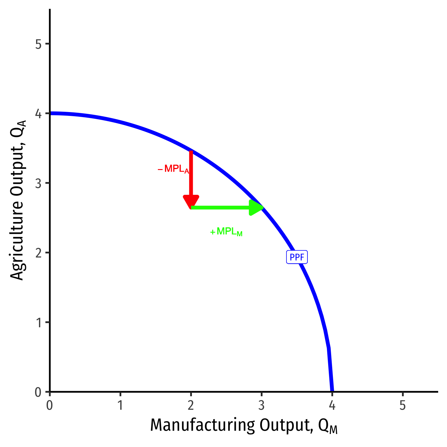
As we move to the right of the PPF, we are pulling labor out of agriculture and into manufacturing
Each single unit of labor we take out of A and put into M will:
- Lower ↓QA by MPLA
- Raise ↑QM by MPLM
Or to put it inversely, to produce 1 more unit of M:
- Reallocate ↓LA input by 1MPLA
- Reallocate ↑LM input by 1MPLM

Production Possibilities Frontier
- Marginal rate of transformation (MRT) increases as we produce more of a good
- Again: “slope”, “relative price of M”, “opportunity cost of M”
- Amount of A given up to get 1 more M
MRT⏟slope=−MPLAMPLM
- Note A(y) on top and M(x) on bottom!†
† This is because, if you think in our Ricardian terms, lx=1MPLx and ly=1MPLy, so lxly⟹MPLyMPLx
Allocating Labor
Because of diminishing returns, as we move labor out of A and into M, we lower MPLM and raise MPLA
This is why the PPF has increasing opportunity costs, and is bent inwards the way it is!
For a given amount of T and L, we can determine the economy's output bundle (QM,QA) by knowing how much labor is allocated across (LM,LA)
Now let's find how labor is allocated across industries
The Demand for Labor in Competitive Industries
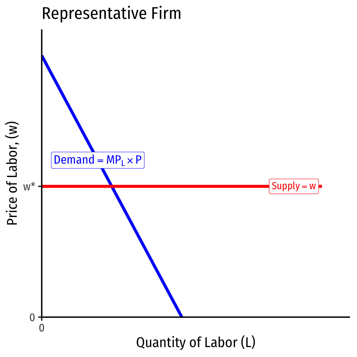
Profit-maximizing firms will hire labor (hours) up to the point where the marginal benefit of hiring labor equals the marginal cost
- Marginal cost per labor-hour: wage w
- Marginal benefit per labor-hour: marginal revenue product (marginal product × price of output)
In manufacturing:
w=MPLM∗PM
- In agriculture:
w=MPLA∗PA
- Again, if you want to remember why, see my slides on Factor Markets
The Demand for Labor in Both Industries
Because we have assumed labor is mobile (and homogenous “labor hours”), workers will always move out of a lower-paying industry and into a higher-paying industry
Thus, in equilibrium, wages w must equalize across both industries, with the implication:
w=MPLM∗PM=MPLA∗PA=w−MPLAMPLM=−PMPA

Labor and the PPF
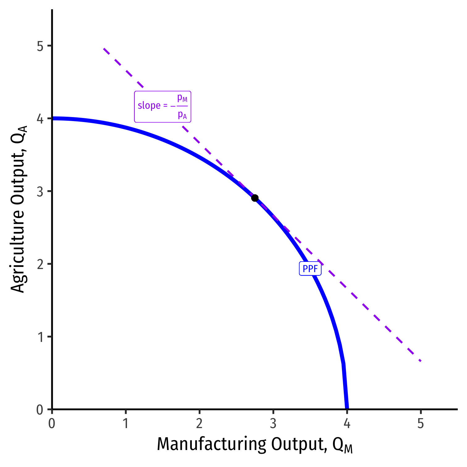
- Thus, we finally see how it is that the slope of the PPF is equivalent to the relative price of M
MRT=−pMpA
(Back to x on top, y on bottom!)
At the optimum production, PPF is tangent to a value line with slope the relative price of M
Labor Allocation
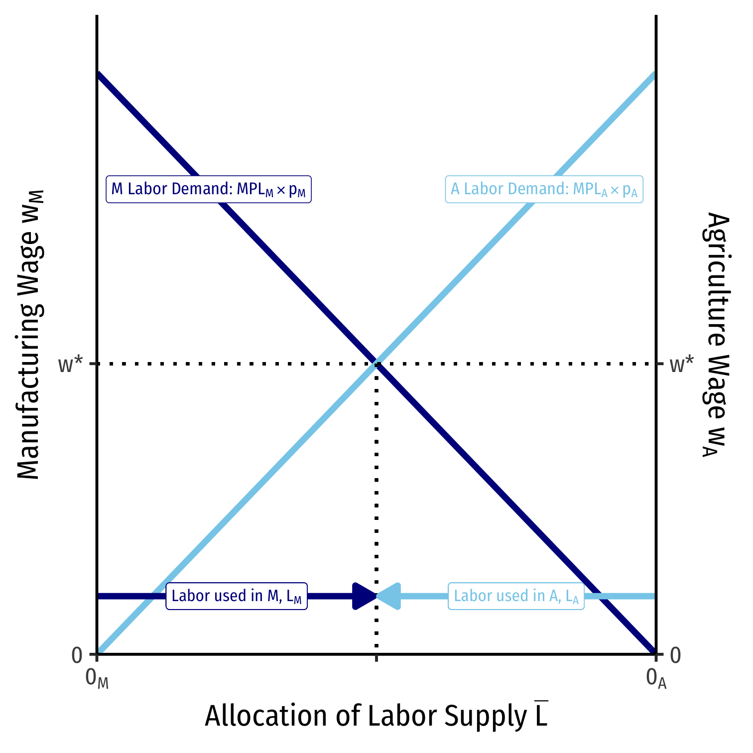
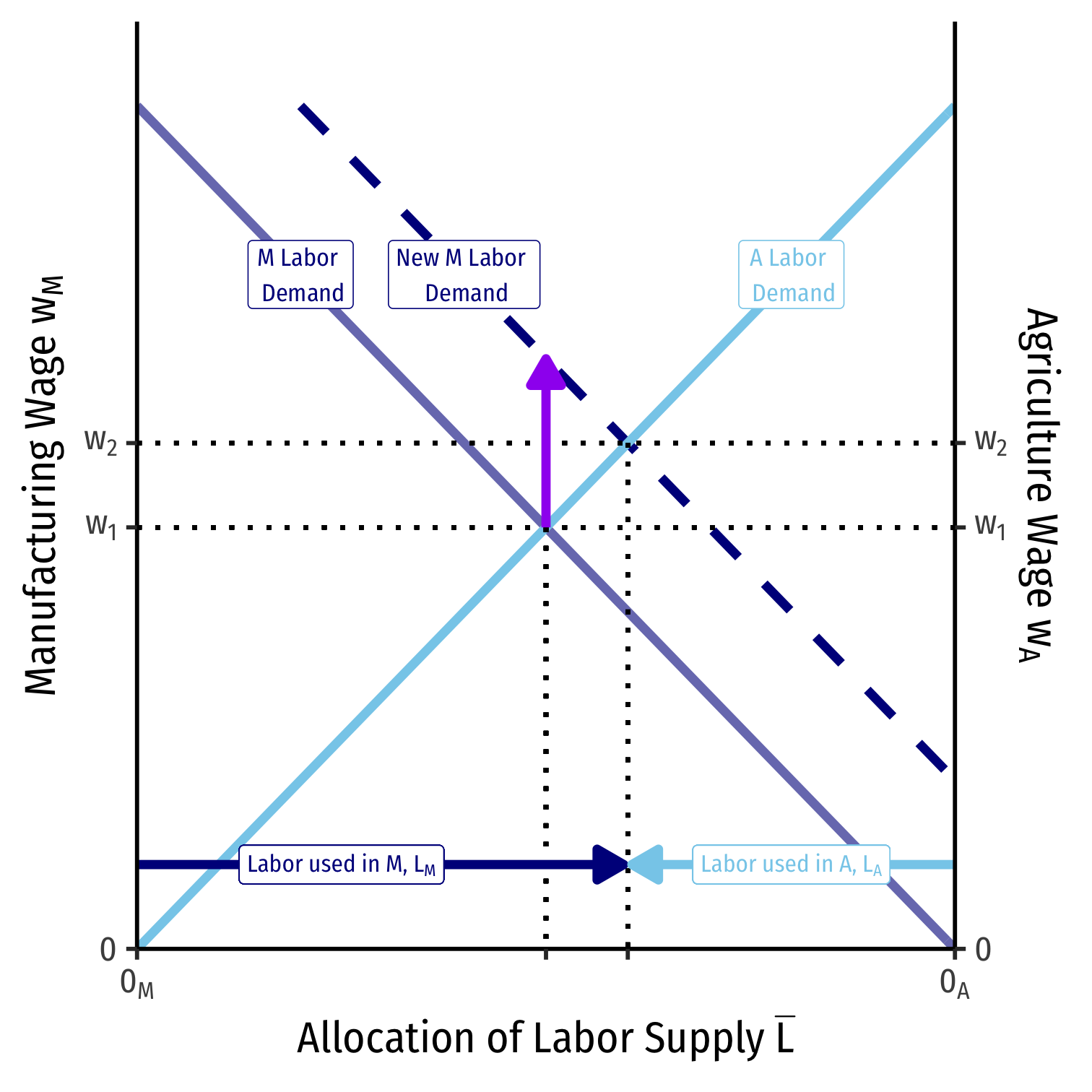
We can also visualize the allocation of labor in the country
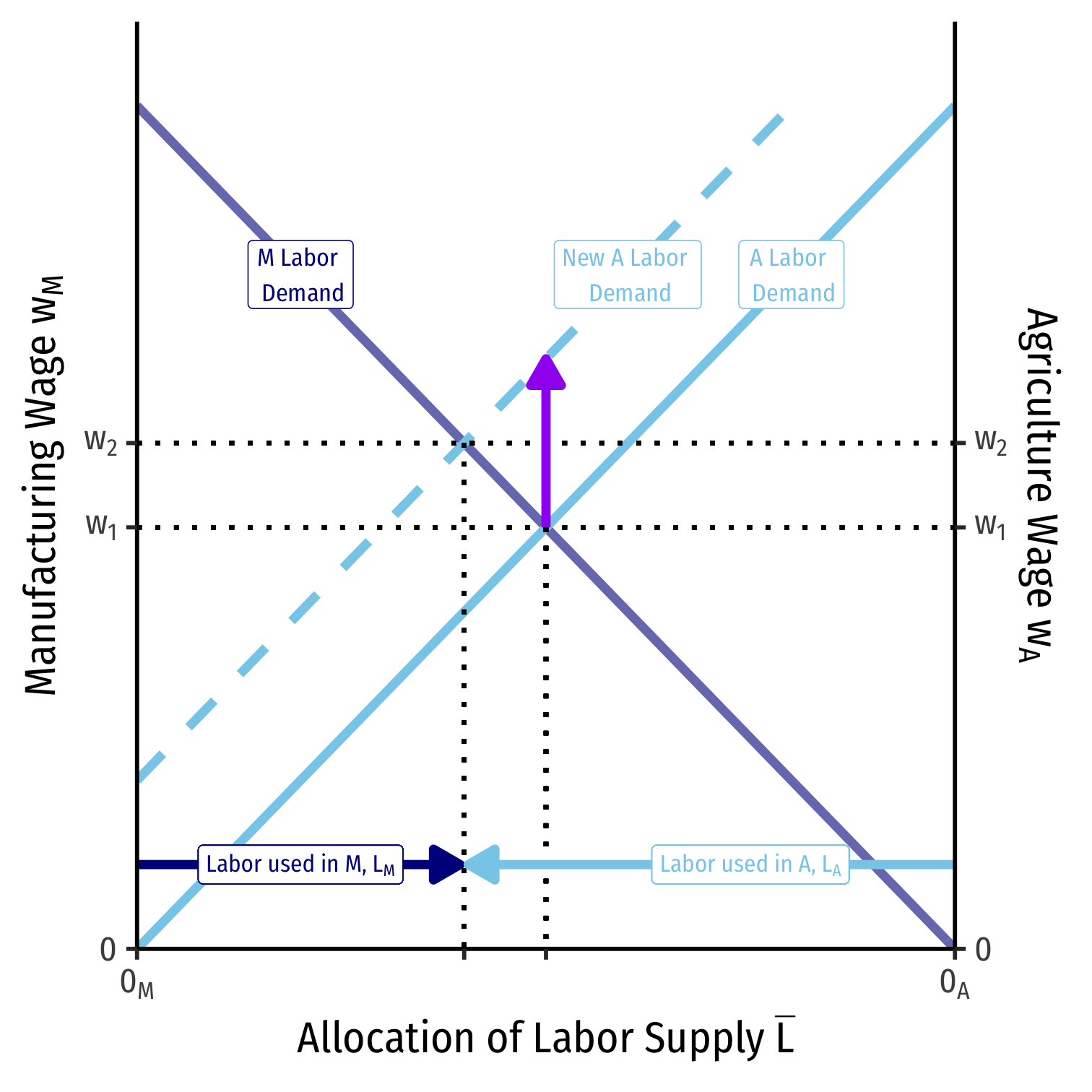
Recall both industries in equilibrium must charge the same wage wM=wA=w⋆
Moving from left to right, labor allocated to manufacturing, LM
Moving from right to left, labor allocated to agriculture, LA
A Change in Relative Prices on Labor Allocation
An increase in the relative price of manufacturing (pMpA) will increase the demand for labor in manufacturing
Because both industries have to compete for labor, wages do increase, but not as much as the increase in the relative price of manufacturing
More labor will be used in manufacturing than in agriculture, and thus, the economy will produce more manufacturing and less agriculture

A Change in Relative Prices on PPF
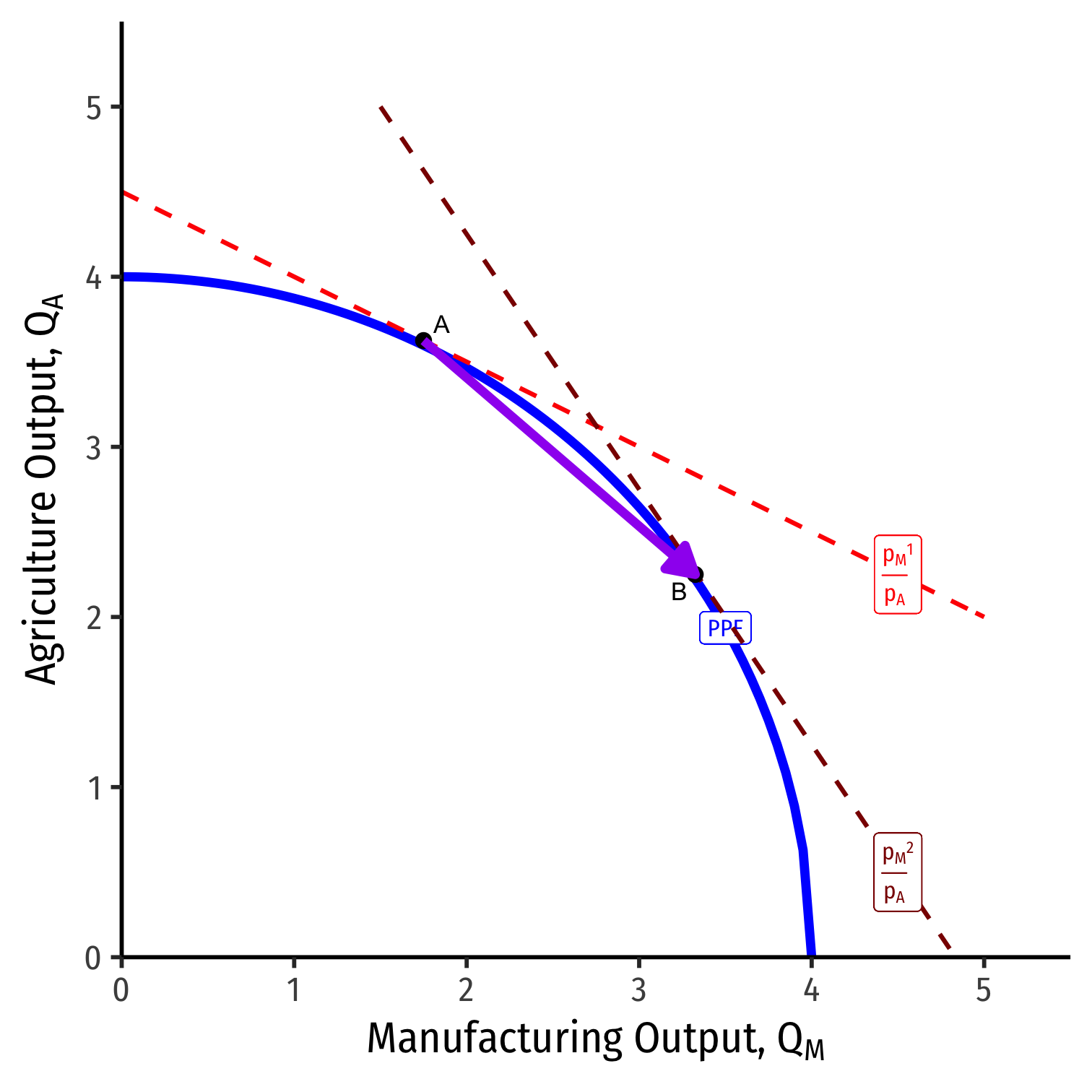
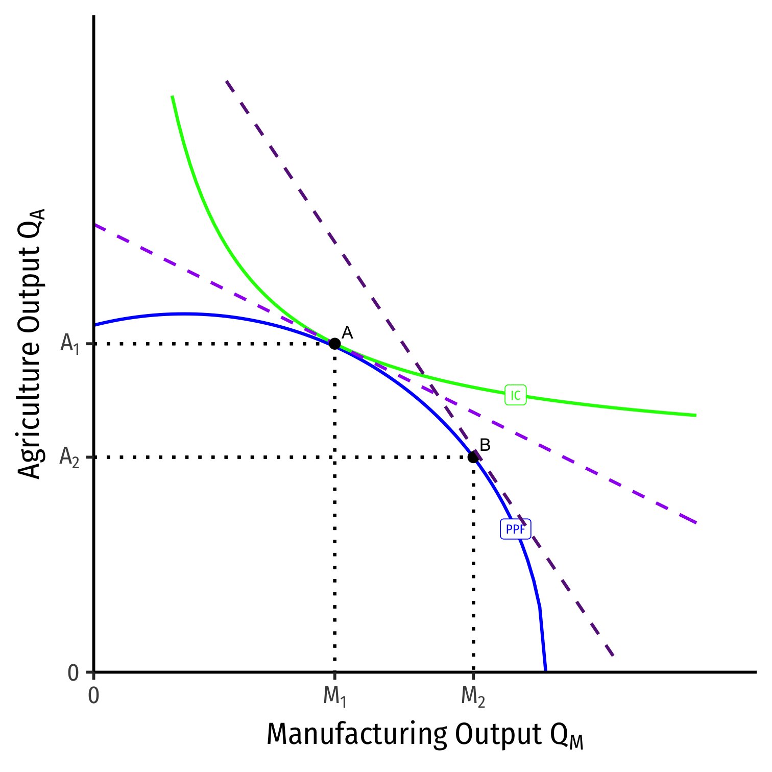
We can equivalently see this on the PPF
Increase in the relative price of manufacturing
(pMpA)1→(pMpA)2
- Moving from A→B
- Slope steepens
- Country will produce less agriculture, more manufacturing
Distribution Effects Using our Two Country Trade Example
Our Two Country Trade Example: Autarky
Home

Foreign
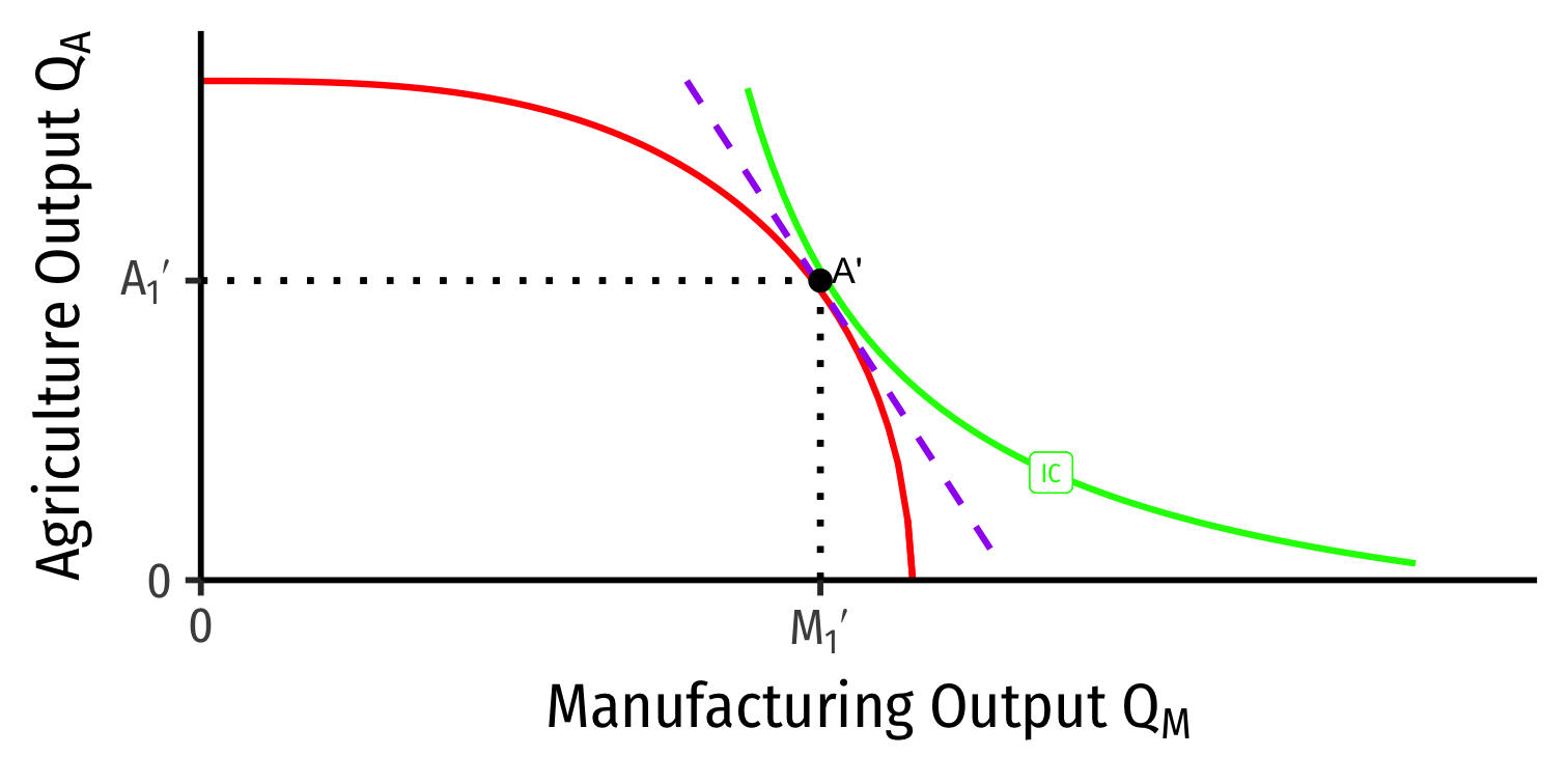
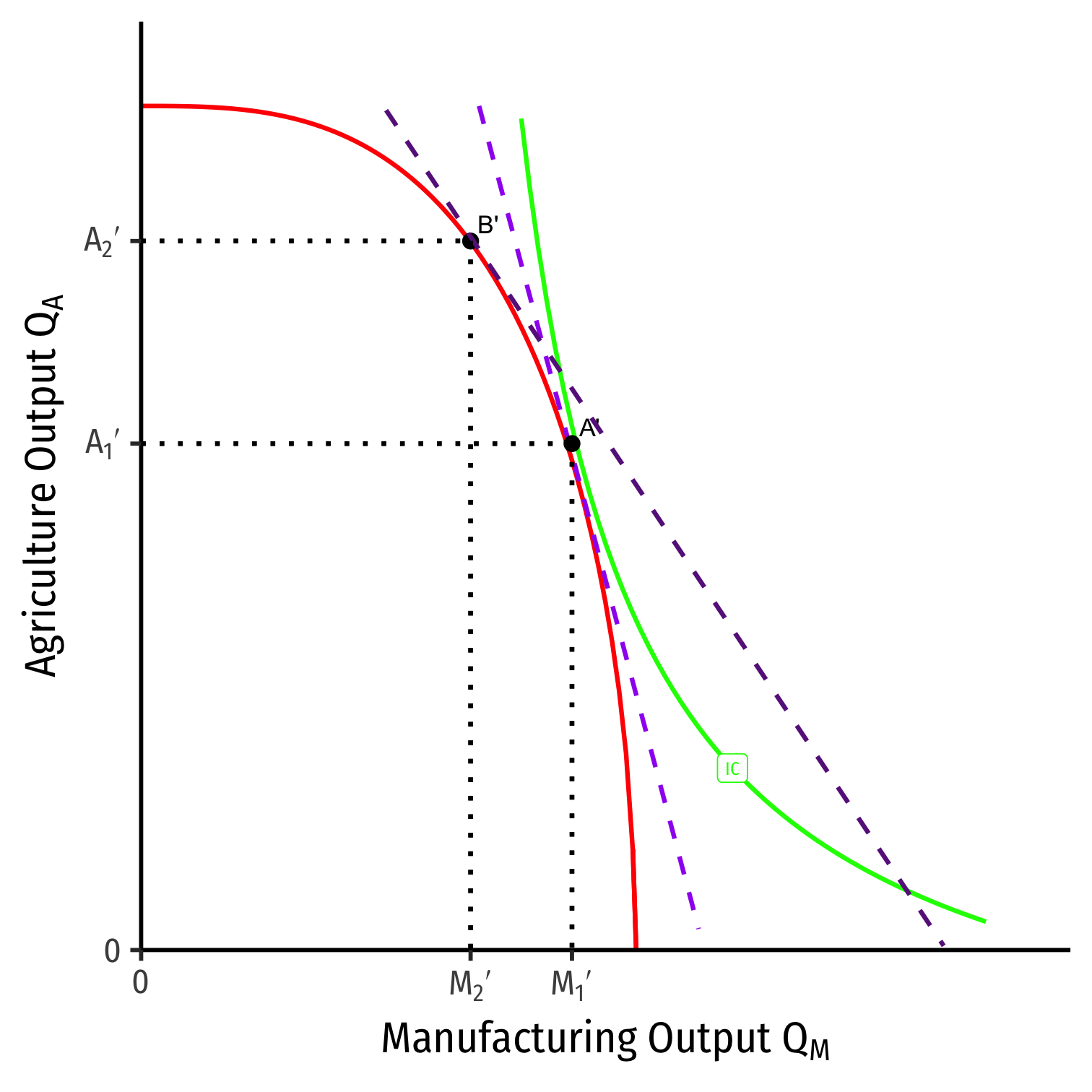
- Countries begin in autarky optimum with different relative prices
- A is optimum for Home
- A' is optimum for Foreign
Our Two Country Trade Example: Specialization
Home
Foreign

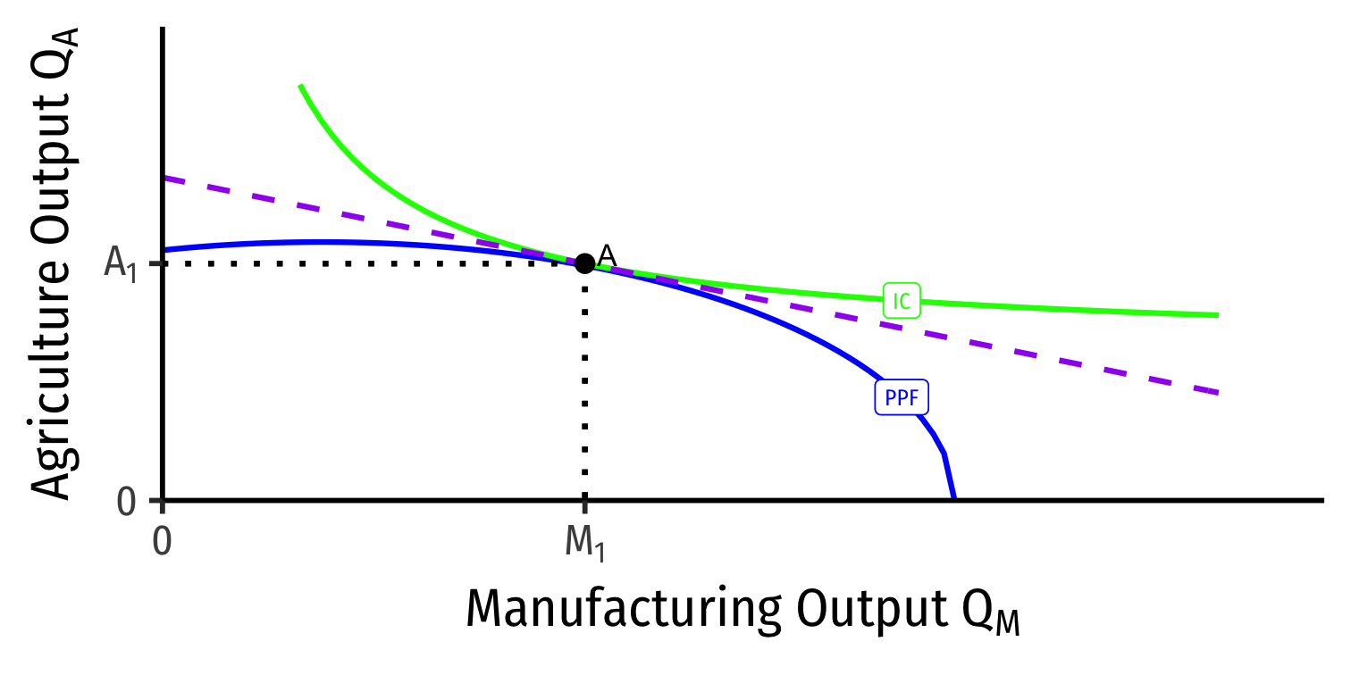
- Home has comparative advantage in manufacturing
- Foreign has comparative advantage in agriculture
Our Two Country Trade Example: Specialization
Home

Foreign
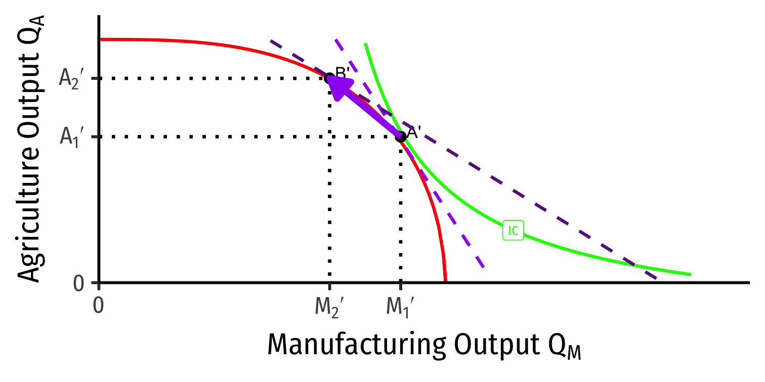
- Countries specialize: produce more of comparative advantaged good, less of disadvantaged good
- Home: A → B: produces more M, less A
- Foreign: A' → B': produces less M, more A
Relative Price Changes in Home
Let's look at three groups at Home:
- Laborers (L)
- Capitalists (owners of K)
- Landowners (owners of T)
Increase in the relative price of manufacturing from trade
- decrease in relative price of agriculture

Effects of Trade on Home's Income Distribution: L
Workers find their wage has increased (but less than increase in relative price of M) Δww1<Δ(PMPA)(PMPA)1
Amount of manufactures QM that can be purchased with wages has fallen!
- Real wage in terms of manufacturing, ↓wpM
Amount of agriculture QA that can be purchased with wages has risen!
- Real wage in terms of agriculture, ↑wpA
Effect on workers is ambiguous
- Depends on their consumption preferences between M and A
Effects of Trade on Home's Income Distribution: K
What about capital owners?
Total income to capitalists =(PM∗QM)⏟Revenues in M−(W∗LM)⏟Labor costs
As more labor used in manufacturing, ↑MPK: Each machine has more workers to work it.
Capital owners gain
- We saw (1) ↑ relative price of manufacturing and (2) ↓ real wage in terms of manufacturing
- Thus, income to capital will rise more than proportionately to the rise in relative price of manufacturing
Advanced Explanation for Capital
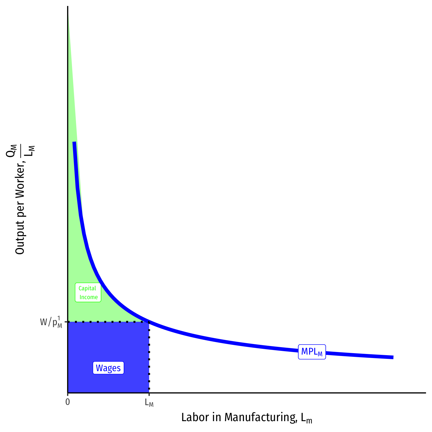
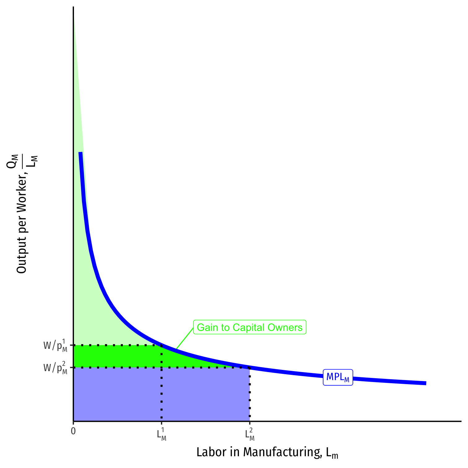
Manufacturing is produced with capital and labor, QM=QM(K,LM)
Total output QM using LM is equal to the under the MPLM curve up to LM
Labor is paid w=MPLM∗pM
- Rewrite as real wage (in terms of M): wPM
- This times the total number of workers LM equals the total wages paid
All residual income goes to capital owners
Advanced Explanation for Capital
Because trade raises the relative price of manufacturing, pMpA, we saw:
- Increase in labor LM, and increase in nominal wage w, but
- Decrease in real wage in terms of m, wpM
Capital owners gain
Effects of Trade on Home's Income Distribution: T
What about land owners?
Total income to landowners =(PAM∗QA)⏟Revenues in A−(W∗LA)⏟Labor costs
As less labor used in agriculture, ↓MPT: Each piece of land has fewer workers to work it.
Land owners lose
- We saw (1) ↓ relative price of agriculture and (2) ↑ real wage in terms of agriculture
- Thus, income to landowners will fall more than proportionately to the fall in relative price of agriculture

Advanced Explanation for Land
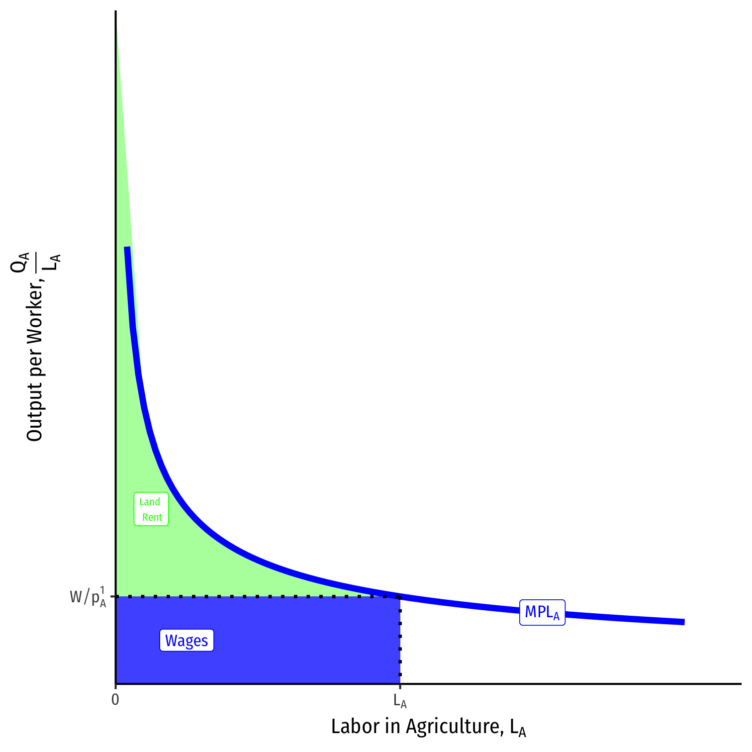
Agriculture is produced with land and labor, QA=QA(T,LA)
Total output QA using LA is equal to the under the MPLA curve up to LA
Labor is paid w=MPLA∗pA
- Rewrite as real wage (in terms of A): wPA
- This times the total number of workers LA equals the total wages paid
All residual income goes to land owners (as rent)
Advanced Explanation for Land
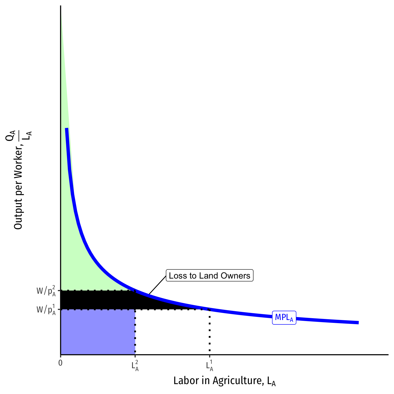
Because trade lowers the relative price of agriculture, pApM, we saw:
- Decrease in labor LA, but increase in nominal wage w, so
- Increase in real wage in terms of A, wpA
Land owners lose
Effects of Trade on Home's Income Distribution
EFfects of trade on Home's:
Labor: ambiguous
- real wage rises in terms of M, falls in terms of A
Capital: income rises more than proportionate to M relative price increase
Land: income falls more than proportionate to A relative price fall

Effects of Trade on Home Income Distribution
Factor specific to the sector whose relative price rises is better off with trade
- Capital for manufacturing
Factor specific to the sector whose relative price falls is worse off with trade
- Land for agriculture
The mobile factor is not clearly better or worse off with trade.
- Labor

Specialization (Again)
Home
Foreign

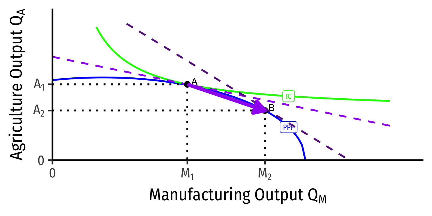
- Countries specialize: produce more of comparative advantaged good, less of disadvantaged good
- Home: A → B: produces more M, less A
- Foreign: A' → B': produces less M, more A
Relative Price Changes in Foreign
Let's look at three groups at Foreign:
- Laborers (L)
- Capitalists (owners of K)
- Landowners (owners of T)
Decrease in the relative price of manufacturing from trade
- increase in relative price of agriculture
Effects of Trade on Foreign's Income Distribution: L
Workers find their wage has increased (but less than increase in relative price of A) Δww1<Δ(PAPM)(PAPM)1
Amount of manufactures QM that can be purchased with wages has risen!
- Real wage in terms of manufacturing, ↑wpM
Amount of agriculture QA that can be purchased with wages has fallen!
- Real wage in terms of agriculture, ↓wpA
Effect on workers is ambiguous
- Depends on their consumption preferences between M and A
Effects of Trade on Foreign's Income Distribution: K
What about capital owners?
Total income to capitalists =(PM∗QM)⏟Revenues in M−(W∗LM)⏟Labor costs
As less labor used in manufacturing, ↓MPK: Each machine has fewer workers to work it.
Capital owners lose
- We saw (1) ↓ relative price of manufacturing and (2) ↑ real wage in terms of manufacturing
- Thus, income to capital will fall more than proportionately to the fall in relative price of manufacturing

Effects of Trade on Foreign's Income Distribution: T
What about land owners?
Total income to landowners =(PA∗QA)⏟Revenues in A−(W∗LA)⏟Labor costs
As more labor used in agriculture, ↑MPT: Each piece of land has more workers to work it.
Land owners gain
- We saw (1) ↑ relative price of agriculture and (2) ↓ real wage in terms of agriculture
- Thus, income to landowners will rise more than proportionately to the rise in relative price of agriculture

Effects of Trade on Foreign's Income Distribution
EFfects of trade on Foreign's:
Labor: ambiguous
- real wage rises in terms of M, falls in terms of A
Capital: income falls more than proportionate to M relative price fall
Land: income rises more than proportionate to A relative price increase

Effects of Trade on Foreign's Income Distribution
Factor specific to the sector whose relative price rises is better off with trade.
- Land for agriculture
Factor specific to the sector whose relative price falls is worse off with trade.
- Capital for manufacturing
The mobile factor is not clearly better or worse off with trade.
- Labor

Takeways from The Specific Factors Model
Takeways from The Specific Factors Model
Changes in trade fall mainly upon the fixed/specific factors of production
- Increase in relative prices (exports) benefit fixed factor producing exports
- Decrease in relative prices (imports) harm fixed factor competing with imports
Mobile factors face ambiguous change
- Can move from low-income industries to high-income industries
Takeways from The Specific Factors Model
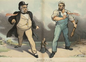
Of course, our simple model aggregates labor into a single mobile factor
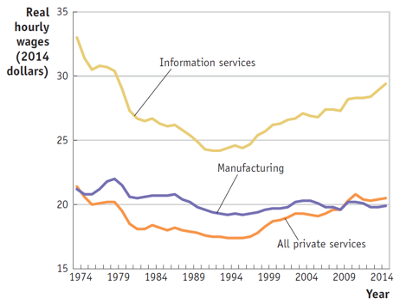
In reality, different types of labor, some may be mobile and some may be immoble and specific
Changes in trade patterns and relative prices will affect specific and mobile factors differently

Example of Mobile vs. Specific Labor
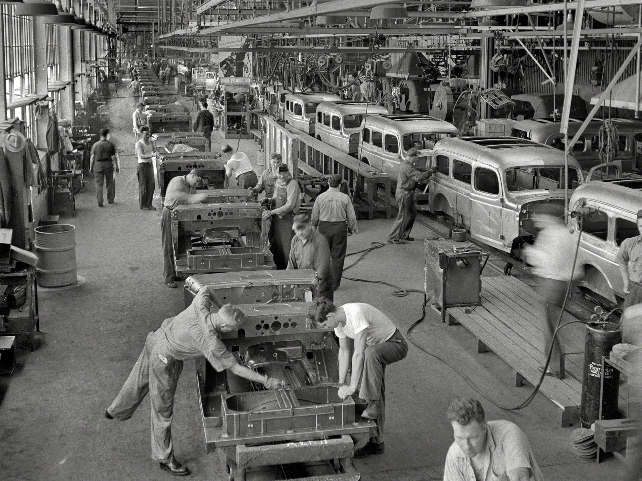
Example: Auto-workers in Detroit in the 1980s were a relatively specific and immobile factor
Geographically concentrated
Skills specific to car assembly-lines

Example of Mobile vs. Specific Labor
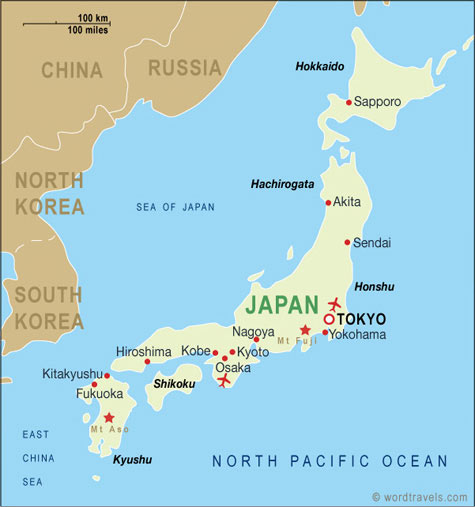
Japan begins exporting cheap cars in 1980s, U.S. consumers import them
Relative price of cars falls in U.S., U.S. factories produce fewer cars, wages & jobs in U.S. auto manufacturing diminish
More mobile and nonspecific workers left Detroit for other industries
- e.g. maybe they went to Texas to work in booming oil industry
More immobile and specific workers lost jobs
- Maybe geographically stuck in Detroit
- Skills were too specific to auto industry, not transferrable to other industries

Some More Examples

Source: Feenstra & Taylor (2017)
Some More Examples
Source: Feenstra & Taylor (2017)
Some More Examples

Source: Feenstra & Taylor (2017)
Takeways from The Specific Factors Model
Again, changes in trade fall mainly upon the fixed/specific factors of production
- Increase in relative prices (exports) benefit fixed factor producing exports
- Decrease in relative prices (imports) harm fixed factor competing with imports
Mobile factors face ambiguous change
- Can move from low-income industries to high-income industries
Policy implication: if governments wish to protect domestic groups from adverse trade shocks, increase mobility and non-specific skills/uses
- make labor, capital, land markets more flexible to reduce shocks from trade on domestic workers, capital-, & land-owners
